


In this tutorial, we are going to illustrate this approach by showing how to reverse-engineer a striking visual illusion using basic math (no more than high school level, promise!) and build an iGLWidget to let you further explore how this illusion works.
Case study: motion induced by the peripheral drift illusion
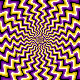
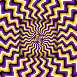
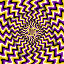
As a case study we picked up the illusion shown below. It has everything a vision scientist likes: it is reasonably complex but tractable, gives a strong sense of illusory peripheral motion, and consists of strong visual cues like contrast, color and depth.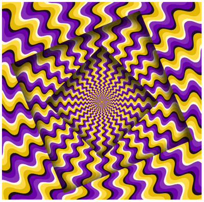
This image can be found on various stock image websites and is credited to Yurii Perepadia, a prolific Ukrainian illustrator and graphic designer who uses Adobe Suite to create his illustrations. He described this one as "Abstract turned frames with a rotating purple yellow wavy pattern". Like for many of his illustrations, Perepadia created the appearance of motion by using an effect studied by Akioshi Kitaoka, a professor of psychology at Ritsumeikan University in Osaka, Japan, and at the basis of his famous "Rotating snakes" illusion: the peripheral drift illusion (PDI). This class of illusions is characterized by the perception of illusory motion when an otherwise static pattern is presented in the peripheral vision while being perceived as motionless when presenting in the center of the visual field. You may notice that the induced illusory motion is particularly strong when exploring the stimulus through eye movements, while it will slow down or even disappear if you are able to stabilize your gaze for a few seconds (this can hard to do though).
Reverse-enginering the illusion
We are going to literally cut this illusion apart to describe its anatomy and try to understand how it works. But no worry, we are not going to use any dangerous tool like scalpel blade, forceps or scissors, but just plain math… and our Psykinematix software. As a reminder, custom stimuli created in Psykinematix can be expressed as a function of up to 4 spatial coordinates (in addition to time, which will not be used here since there is actually no moving part in this illusion):z = f( x ,y, r, theta, time)
| where (x, y) are the Cartesian coordinates and (r, theta) are the polar coordinates of each pixel P of the stimulus (x being its horizontal position relative to the center O, y its vertical position relative to O, r its distance to O, and theta the angle defining its counterclockwise direction relative to the x axis). z is simply the evaluation of the f () function as a 2D output between 0 and 1 to represent the normalized luminance of each pixel. For colored pixels, we will use outputs designated zr, zg and zb also between 0 and 1 to represent the normalized luminance of its red, green and blue chromatic components. For f (), we will only use a combination of basic mathematical functions like arithmetic operations, trigonometric functions, and comparison operations, as well as a number of intermediate variables. Note that while using both Cartesian and polar coordinate systems is redundant to express the pixel location, they can be handy to describe different components of this stimulus as we will see later. | 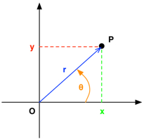 |
This complex pattern is made of various components whose contribution for the strong illusory motion may be difficult to discern at first. The pattern can be summarily described as yellowish "tentacles" on a purple background spreading in the radial direction and uniformly spaced in the angular direction, and split into 3 different depths seen through 2 central squarish windows rotated and increased in size. Let's describe mathematically each of those components.
Spatial pattern
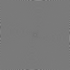
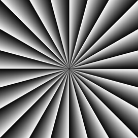
First let's focus on the main spatial feature of this illusion: its 24 sprawling components uniformly spaced by 15 degrees (360/24). The simplest expression to create this basic distribution is a sinusoidal luminance grating in the angular direction as illustrated below: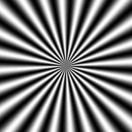
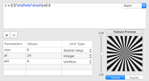
where theta indicates the angular position and af expresses the number of wedges per circumference (or angular frequency). phi is an optional angular phase parameter to rotate the whole pattern by some arbitrary angle. With Psykinematix, you simply need to enter this expression in the custom stimulus section to see what the stimulus looks like and how its appearance is affected when changing the value of the parameters.
The curvature of these "tentacles" can be modulated by applying some clever value to the phi parameter. For example replacing phi with the radial position of each pixel (i.e. the variable r) produces an angular shift that grows linearly with the radial direction (i.e. away from the pattern center) hence forming a spiral distortion of the tentacles as illustrated below.
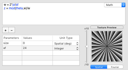
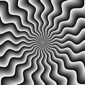
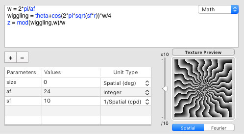
Wiggles along the radial direction (i.e. with angular shifts alternating between positive and negative values, or left and right) can be created with a sinusoidal modulation of the angular shift as a function of the radial position r :
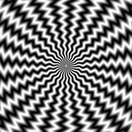
where sf is the spatial frequency of the wiggling along the radial direction (the higher this value the smaller the distance between 2 consecutive wiggles).
Color sequence
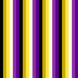
If one inspects carefully each tentacle, one would notice that the color modulation in the angular direction is not continuous but rather consists of 6 discrete colors that alternate in a cyclic manner with the following r,g,b coordinates: black (0, 0, 0), dark orange (0.8, 0.7, 0), light orange (1, 0.9, 0.3), almost white (1,1,0.9), light purple (0.6, 0.2, 0.7) and dark purple (0.4, 0, 0.6).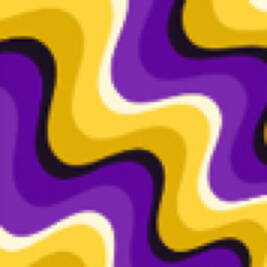
While the sinusoidal luminance grating we used above provides a first approximation of the tentacles shape, it cannot account for the luminance and color variation in the pattern: a sinusoidal wave alternates smoothly from dark, grey, white, and grey again in a cyclic manner. To account for the original pattern, one needs to create 6 unique colors which cannot be obtained from a one-to-one mapping of a sinusoidal cycle. One should instead consider a sawtooth modulation function giving 6 discrete indices (0, 1, 2, 3, 4, and 5) which can then be used to specify each color (e.g. 0 for black, 1 for dark orange, 2 for light orange, 3 for white, 4 for light purple and 5 for dark purple).
As illustrated below, such a colorful sawtooth function can be simply produced by applying the modulo operation mod() along the direction of color change (the x axis in this example) and comparing the result of this operation to an index used to select the (r, g, b) components of the associated color:
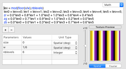
where w is a parameter to set the width of each colored band. Note that for each given pixel, only one of the variables lev* takes a value of 1 and all other variables lev* take a value of 0, so the output variables zr, zg and zb will always be set to one of the 6 picked colors for each pixel. We will refer to this selection technique as the index-based color picking.
One can replace the sinusoidal function with a sawtooth function to produce a similar tentacular pattern which is more appropriate for the above color picking:
One could note that this is very similar to the basic pattern found in one of the first studies that discovered the peripheral drift illusion: the basic illusory motion can be simply generated with a sawtooth luminance grating presented in the visual periphery (Faubert and Herbert, 1999).
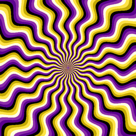
The wiggling can be produced similarly to above by incorporating a sinusoidal modulation of the angular shift as function of the radial position:
We finally obtain the colorful wiggling tentacles by applying a sampling with 6 levels on the luminance profile of this sawtooth modulation and the index-based color picking:
Congratulations if you are still there, the most difficult part is done! Now let's move on to the square windows.
Spatial envelopes
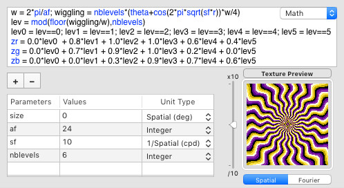
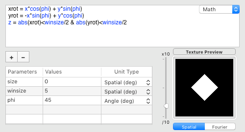
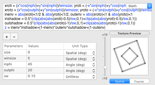
In the original illustration, the above tentacular pattern appears to be replicated at different depths seen through 2 see-through square windows.A square can be simply created by checking whether both x and y positions are within its border (where the variable winsize denotes here the length of its sides):

The smallest and deepest square in the original illustration is actually rotated by 45 deg (phi variable). This transformation can be obtained by applying the standard formulas for rotating the x-y axes:

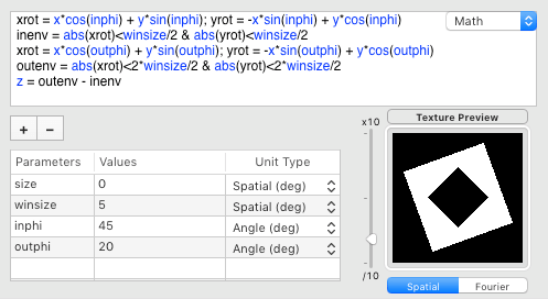
The largest and closest square is about twice larger and rotated by about 20 deg (outphi variable). The middle depth plane is simply this larger window (outenv) minus the smaller one (inenv):

If you look closely at the borders of the see-through windows in the original image, you will notice that the order of the color sequences of the tentacles in the middle depth plane is inverted compared to the inner and outer ones which may further enhance the strength of the illusion through the creation of antagonism illusory motion:
|
 |
Those index changes can be computed with the following sub-expression:
mod(nblevels-levels,nblevels)
This color order inversion is then only applied to the middle depth plane using the above mask when computing the color indices:
We are almost there ! Something is however still missing: the perception of depth…
Depth
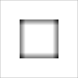
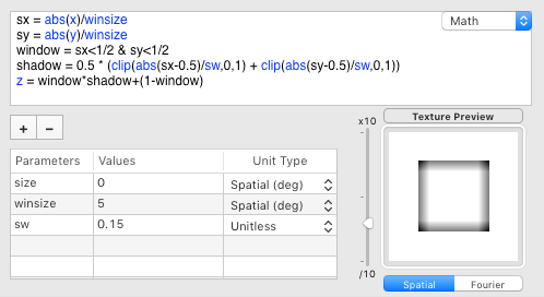
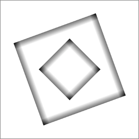
Depth perception can be typically enhanced by the presence of shadows. But shadows alone can also provide strong depth cues. Here one would expect the windows borders to cast some shadow (penumbra) on the patterns behind them. Shadows can be created simply by darkening the stimulus luminance inside the edges of the windows (for simplicity here, we are only assuming some ambient lightning and no directional light source). Realistic shadows should also smoothly attenuate with the distance from the edges.This can be simulated through a linear increase of the luminance modulation as function of the distance to each edge as illustrated below, where the amount of shadowing is controlled by a single parameter sw that specifies the spatial extent of this modulation (i.e. how far from the edges it spreads):
Let's apply this shadow on a single windowed view of our wiggling stimulus:
We have now a much more convincing perception of depth !
The same technique can apply to the 2 inner and outer rotated windows:
Then we finally obtain a stimulus very similar to the illustration created by Yurii Perepadia:
Widget
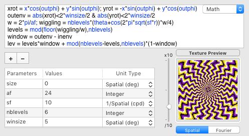
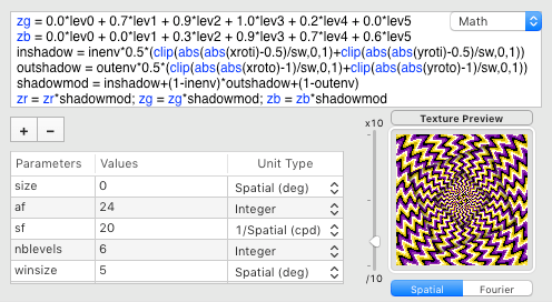
Here is the final mathematical expression: # Useful pre-computation for some parameters
inphi = 45*pi/180
sw = shadow/100
w = 2*pi/af
# Spatial pattern: wiggling tentacles
wiggling = nblevels*(theta+cos(2*pi*sqrt(sf*r))*w/4)
# Rotated inner and outer square windows
xroti = (x*cos(inphi)+y*sin(inphi))/winsize
yroti = (-x*sin(inphi)+y*cos(inphi))/winsize
inenv = abs(xroti)<1/2 & abs(yroti)<1/2
xroto = (x*cos(outphi)+y*sin(outphi))/winsize
yroto = (-x*sin(outphi)+y*cos(outphi))/winsize
outenv = abs(xroto)<1 & abs(yroto)<1
# Luminance discretization
levels = mod(floor(wiggling/w),nblevels)
# Selection of middle depth plan
window = outenv - inenv
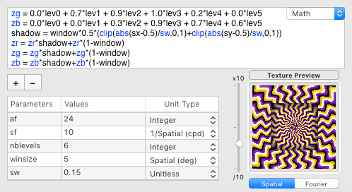
# Color picking with inversion for middle depth plan
lev = levels*window + mod(nblevels-levels,nblevels)*(1-window)
lev0 = lev==0; lev1 = lev==1; lev2 = lev==2 ; lev3 = lev==3; lev4 = lev==4; lev5 = lev==5
zr = 0.0*lev0 + 0.8*lev1 + 1.0*lev2 + 1.0*lev3 + 0.6*lev4 + 0.4*lev5
zg = 0.0*lev0 + 0.7*lev1 + 0.9*lev2 + 1.0*lev3 + 0.2*lev4 + 0.0*lev5
zb = 0.0*lev0 + 0.0*lev1 + 0.3*lev2 + 0.9*lev3 + 0.7*lev4 + 0.6*lev5
# Shadows
inshadow = inenv*0.5*(clip(abs(abs(xroti)-0.5)/sw,0,1)+clip(abs(abs(yroti)-0.5)/sw,0,1))
outshadow = outenv*0.5*(clip(abs(abs(xroto)-1)/sw,0,1)+clip(abs(abs(yroto)-1)/sw,0,1))
shadowmod = inshadow + (1-inenv)*outshadow + (1-outenv)
# Final result
zr = zr*shadowmod
zg = zg*shadowmod
zb = zb*shadowmod
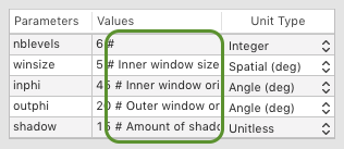
1) you specify which parameters should be controllable, their labels, the range of the values available from their slider controls and their units. This can be specify by adding some metadata after the default value of each parameter (following the # symbol) as highlighted below:
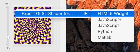
2) then control-click on the preview and select the GLSL export option "HTML5 Widget",
3) finally you enter in the widget configurator panel the optional detailed information to appear in the back side of the widget,
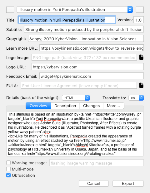
4) and click the "Export" button to produce a ready-to-use HTML5 widget that can be shared with others either online or offline on any platform.
And here it is the iGLWidget for this illusion exported from Psykinematix Pro Edition that lets you play in real-time with some of its parameters. You will notice that we added 2 parameters, saturation and contrast. We leave their implementation as an exercise, but you can find the solution somewhere in the back side of the widget below… Enjoy !
This widget will be part of our second set of iGLWidgets to be released soon, which will be dedicated to some classical visual illusions. To learn more, feel free to explore our public iGLWidgets Collection for Vision Science.
If you have any comment or question about this tutorial, please post them in the comments section on our Psykinematix Twitter account or Facebook group or private message us from there !
William H.A. Beaudot
KyberVision Japan LLC (Sendai, Miyagi)
References
Fraser & Wilcox (1979) Perception of illusory movement. Nature 281:565–566
Faubert & Herbert (1999) The peripheral drift illusion: A motion illusion in the visual periphery. Perception 28:617–621
Kitaoka & Ashida (2003) Phenomenal characteristics of the peripheral drift illusion. Vision (15):261–262
Publish Date: 31 August 2020